
 Back
Back 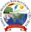

Energy & Wetlands Research Group, Center for Ecological Sciences [CES],
http://ces.iisc.ac.in/energy
Centre for Sustainable Technologies (astra)
Centre for infrastructure, Sustainable Transportation and Urban Planning [CiSTUP],
Indian Institute of Science, Bangalore, Karnataka, 560 012, India
Abstract
Global warming with the escalation in greenhouse gas (GHG) footprint (400 parts per million from 280 ppm CO2 emissions of the pre-industrial era) and consequent changes in the climate has been affecting the livelihood of people with the erosion of ecosystems productivity. The anthropogenic activities such as power generation (burning of fossil fuels), agriculture (livestock, farming, rice cultivation and burning of crop residues), polluting water bodies, industry and urban activities (transport, mismanagement of solid and liquid waste, etc.) have risen substantially CO2 concentrations to 72% among greenhouse gases. Emissions and sequestration of carbon need to be in balance to sustain ecosystem functions and maintain the environmental conditions. Forests are the major carbon sinks to mitigate global warming. The current research focusses on the carbon budgeting through quantification of emissions and sinks in the Uttara Kannada district, central Western Ghats, Karnataka. This would help in evolving appropriate mitigation strategies towards sustainable management of forests. The study reveals that total carbon stored in vegetation and soils are 56911.79 Gg and 59693.44 Gg respectively. The annual carbon increment in forests is about 975.81 Gg. Carbon uptake by the natural forest is about 2416.69 Gg/yr and by the forest plantations is 963.28 Gg/yr amounting to the total of 3379.97 Gg/yr. Sector wise carbon emissions are 87.70 Gg/yr (livestock), 101.57Gg/yr (paddy cultivation), 77.20 Gg/yr (fuel wood consumption), 437.87 Gg/yr (vehicular transport) respectively. The analysis highlights that forest ecosystems in Uttara Kannada are playing a significant role in the mitigation of regional as well as global carbon emissions. Hence, the premium should be on conservation of the remaining native forests, which are vital for the water security (perennial streams) and food security (sustenance of biodiversity) and mitigation of global warming through carbon sequestration. Sustainable management ecosystem practices involving local stakeholders will further enhance the ability of forests to sequester atmospheric carbon apart from other ecosystem services, such as hydrological services, improvements in soil and water quality.
Keywords: Carbon sequestration, emissions, forest ecosystems, carbon budgeting, sustainable management
 |
Introduction
Forests sequester atmospheric carbon (Gallaun et al. 2010; Pan et al. 2011) and play a pivotal role in mitigating changes in the climate (Jackson and Baker 2010; Dymond et al. 2016). Atmospheric carbon gets stored in the above and below ground biomass and soil organic matter. Mismanagement of forests leading to deforestation and enhanced anthropogenic emissions during post industrial revolution has increased carbon dioxide concentration in the atmosphere to 400 ppm from 270 ppm during the pre-industrial era (Manua Loa, 2017). The recent estimates of emissions in 30 developing countries (including Brazil, Bolivia, Indonesia, Myanmar and Zambia) highlight that deforestation and forest degradation are the prime sources of CO2 imperiling productive ecosystems (Edgar, 2011). Carbon dioxide, nitrous oxide, methane, chlorofluorocarbon and water vapors are major greenhouse gases (GHG), which induce greenhouse effect by absorbing and re-emitting infrared radiation in Earth's atmosphere. This has resulted in the increase of the earth's ambient temperature, leading to global warming, with the consequent changes in the climate impacting the survival of living organisms. Carbon footprint is thus a measure of the impact of human activities on the environment in terms of the amount of greenhouse gases produced and expressed in units of carbon dioxide equivalent (CO2 Eq). The amount of carbon storage or sequestration is expressed as amounts in metric tons or Gg (Giga gram) per hectare, which indicates the amount of carbon uptake by forests. The effective forest management greatly influences the amount of carbon stored in the aboveground biomass, soils, and associated forest products.
Burgeoning population and unplanned urbanisation coupled with the increased consumption levels have led to the release of a large amount of carbon from anthropogenic sources. Deforestation and forest degradation accounts to 20â25% of the total anthropogenic carbon emissions (Pachauri and Reisinger 2007). Vegetation store the carbon in the form of carbohydrate and soil accumulate the carbon in organic and inorganic form. Forest removal leads to the release of stored carbons and the global phenomenon of deforestation have contributed to an increase in atmospheric CO2. Large scale land use land cover (LULC) changes leading to deforestation, indiscriminate harvesting of industrial wood, forest fire, etc. are responsible for carbon emissions. LULC changes modify biogeochemical cycles, climate, hydrology (Bharath et al. 2013; Regos et al. 2015; Vinay et al. 2017), driving biodiversity loss through habitat fragmentation and destruction (Sala et al. 2000; Sharma et al. 2016). Irrational LULC changes have been posing challenges with alterations in the ecosystem integrity leading to the decline of ecosystem services, which is affecting the livelihood of people. India emits nearly 5% of global CO2 emissions, which is expected to increase by more than 2.5 times by 2030 (IEA 2010). This necessitates the quantification of sources and sinks of carbon in order to evolve appropriate mitigation and adaptation strategies. Carbon budgeting of a region provides the spatial and temporal distribution of major pools of carbon sources and sinks that help in assessing the pattern and variability of carbon in the atmosphere. Terrestrial, aquatic plants and soil are major carbon sinks, which accumulate the carbon. Sources of GHG for a region are from livestock, agriculture, fuelwood consumption, industries, transportation, land use changes, etc. The carbon budget of a region (United Nations Framework Convention on Climate Change, UNFCCC) include emissions from burning fossil fuels, industrial production, direct emissions from heating in households and businesses, transportation, agriculture, waste management, land use, forestry and emissions arising from other activities.
1.1 Objectives
The objective of the current research is to carry out taluk wise carbon budget for Uttara Kannada district, Central Western Ghats. This involves,
- Source wise carbon sequestration assessment with the combination of field and remote sensing data.
- Sector wise assessment of carbon emissions
- Computation of regional level carbon metric (ratio of carbon sink to source).
|
2.Materials and Method
2.1 Study area
The Western Ghats or or "Sahyadri" is a chain of mountains ranges along the western side of India is one among the global ten "Hottest hotspot of biodiversity". Uttara Kannada with an area of 10,291 sq. km (covering 5.37% of Karnataka state) is located between 13.769o to 15.732o north and 74.124o to 75.169o east (Fig. 1) in the central part of the Western Ghats. The district extends to about 328 km north to south and 160 km east-west is hilly, undulating and thickly wooded and comprises of 11 taluks (also known as tehsil - an area of land with a city or town that serves as centre local administrative unit in south Asian countries). The region consists of three agro-climatic zones namely coastal, hilly and plains. The soils of the district are divided into distinct zones based on topography; the alluvial, lateritic and granitic soils. The soil can be described as derivatives of the most ancient metamorphic rocks in India, which are rich in iron and manganese (Pascal 1988). Forests of Uttara Kannada are broadly divided into moist and dry types. The moist type may be subdivided into evergreen, semi evergreen and moist deciduous. The dry type can be divided into dry deciduous and thorn forest. The central part of Uttara Kannada is of the evergreen type. The total population of the district is 1436847 with density as 140 persons per sq.km. The agricultural sector has been playing a prominent role in the economy evident from the production of crop varies such as paddy (182000 metric tons); sugarcane (45000 metric tons), groundnut (4695 metric tons) and horticulture crops production accounts to 179671 metric tons.
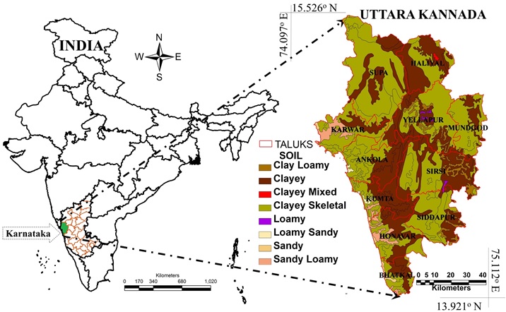
Fig. 1 Study region - Uttara Kannada district, Central Western Ghats
2.2 Method
Fig. 2 outlines the approach adopted for budgeting carbon in Uttara Kannada. Forest types are mapped using vegetation maps (Pascal 1986; Ramachandra et al. 2016), field data with the remote sensing data. Forest vegetation is sampled using transect-based quadrats (Fig. 3), which is validated and found appropriate especially in surveying undulating forested landscapes of central Western Ghats (Chandran et al. 2010; Ramachandra et al. 2015a,b). Topographic maps of 1:50000 scales were used to do ground surveys and selection of sample plots. Availability of temporal remote sensing data helped in understanding the vegetation dynamics and in assessing biomass and carbon uptake. Further, the analysis was carried out in two major folds i.e., spatial mapping of carbon sinks, estimating carbon emissions.
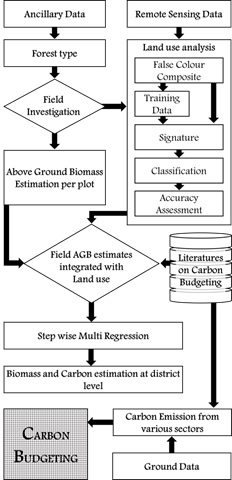
Fig. 2 Method adopted for carbon budgeting
2.2.1 Land Use (LU) dynamics
LU analysis of a region provides the status of a landscape and its health. Land use changes induced by human activities play a major role at global as well as at regional scale climate and biogeochemistry of the Earth system. These changes directly impact biodiversity of a region (Ramachandra et al. 2018), soil degradation, loss of CO2 sequestration potential, which induce local climate change (Silva et al. 2016) as well as global warming (Wei et al. 2014). Earlier studies have revealed deforestation and other LU change activities are the prime agents of atmospheric CO2 increase (Ciais et al., 2013) and consequent global warming. The temporal LU analyses provide insights to the rate of CO2 emissions escalation with deforestation and loss of carbon sequestration potential of the ecosystem (Quere et al. 2015). LU combining with 'ground based' in situ data serves as a cost-efficient and reliable source to account carbon emissions (Hooijer et al. 2010; Mohren et al. 2012). Land use analyses involved (i) generation of False Color Composite (FCC) of RS data (bandsâgreen, red and NIR). This composite image helps in locating heterogeneous patches in the landscape, (ii) selection of training polygons by covering 15% of the study area (polygons are uniformly distributed over the entire study area) (iii) loading these training polygons co-ordinates into pre-calibrated GPS, (vi) collection of the corresponding attribute data (land use types) for these polygons from the ï¬eld, (iv) supplementing this information with Google Earth and (v) 60% of the training data has been used for classiï¬cation based on Gaussian Maximum Likelihood algorithm, while the balance is used for validation or accuracy assessment (ACA). The land use analysis was done using a supervised classification technique based on Gaussian maximum likelihood algorithm with training data. The land use is classified under 11 categories such as Built-up, Water, Cropland, Open fields, Moist deciduous forest, Evergreen to semi evergreen forest, Scrub/grass, Acacia/Eucalyptus/ Hardwood plantations, Teak/ Bamboo/ Softwood plantations, Coconut/ Areca nut/ Cashew nut plantations, Dry deciduous forest. GRASS GIS (Geographical Resources Analysis Support System, http://ces.iisc.ac.in/grass) - free and open source software has been used for analyzing RS data by using available multi-temporal âground truthâ information. Earlier time data were classified using the training polygon along with attribute details compiled from the historical published topographic maps, vegetation maps, revenue maps, land records available from local administrative authorities. The Landsat data of 1973 with a spatial resolution of 57.5 m à 57.5 m (nominal resolution) were resampled to 30 m (nominal resolution) to maintain the uniform resolution across temporal (1999-2018) RS data.
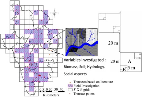
Fig. 3 Study area and distribution of transects cum quadrats for sampling vegetation
2.2.2 Spatial mapping of carbon sinks
The study area falls in three agro-climatic regions. The district is is divided into 5'*5' equal area grids (168) covering approximately 81 km2 (9*9 km) comparable to grids in the Survey of India topographic map (of 1:50000 scale). Representative grids were chosen in each agro-climatic zone for further field data collections (Fig. 3). The basal area, height, species type, diversity, etc. were computed based on the collected field data through flora sampling in quadrats of 116 transects (distributed across agro-climatic zones). Along a transect of 180 m, 5 quadrats each of 20 m *20 m were laid alternately on the right and left, for tree study (minimum girth of 30 cm at GBH (girth at breast height or 130 cm height from the ground) and height > 1.5 m), keeping intervals of 20 m length between successive quadrats. Two sub-quadrats of 5 m *5 m were laid within each tree quadrat, at two diagonal corners, for shrubs and tree saplings (<30 cm girth). Within each of these, 2 herb layer quadrats each of 1 sq.m area, were laid for documenting herbs and tree seedlings. Standing biomass in forests and plantations is quantified to evaluate carbon sequestration potential of the respective ecosystem. Land use analysis is performed to account grid wise and at district level forest cover, which helped in estimating biomass at the district level.
2.2.3 Quantification of biomass (Forests)
The above ground biomass (AGB) of trees refers to the cumulative weight of the tree biomass above ground, in a given area. The change in standing biomass over a period of time is called productivity (which is assessed based on biomass increment monitoring for 36 months, thrice during the past three decades). AGB is a valuable measure for assessing changes in forest structure (Brown et al. 1999; Cummings et al. 2002) and an essential aspect of studies of the carbon cycle. AGB data at a landscape scale can be used to understand changes in forest structure resulting from succession or to differentiate between forest types (Cairns et al. 2003). AGB was calculated using the basal area equation and below ground biomass calculated from indirect estimation (Chandran et al. 2010; Ramachandra et al. 2000a; Murali et al. 2005; Ravindranath et al. 2008). The region specific allometric equations (Table 1) have been used to compute biomass (Chandran et al. 2010; Brown 1997). The study area falls in three diverse agro climatic variations i.e. Coastal; Sahyadri Interior; Plains. Probable relationship between basal area (BA), and forest cover and extent of interior forest (equation 1) based on the field data coupled with land use data. The multiple regression analysis is done for estimating the relationship between a dependent (standing biomass) and independent variables (basal area, forest cover, percentage of interior forests-computed from land use analysis). The probable relationship as per eq. 1, was used for predicting the standing biomass and carbon stock in all grids.
Standing biomass= F{basal area,interior forest,forest cover} ....1
Statistically significant equations based on the basal area with land use and interior forest were obtained and given in equations 2, 3, and 4 respectively for coastal, Sahyadri and plains. Validation of basal area based on equation 2-4 was done with the known basal area (colleted through field sampling) in the respective grids (Fig. 6). Later, basal area (Table 2) for all grids in the coast, Sahyadri interior and plains were computed considering forest land use and interior forests (in the respective grids) using equations 2, 3 and 4.
For Coastal regions,
BA={30.1+(0.0414*(forest land use)+0.053*(interior forest))};
n=50, SE=6.2 ...2
For Sahyadri Interior region,
BA={39.1+ (-0.099*(forest land use)+0.091*(interior forest))};
n=55, SE=6.3 ...3
For plain region,
BA={34.8+ (-0.186*(forest land use)+0.12*(interior forest))}; ;
n=11, SE=5.5& nbsp; ...4
Where n is a number of transects and SE refers to standard error. Comparisons of predicted (as per equations 2,3 and 4 for different agro-climatic regions) and quantified basal area from the field showed a reasonable agreement with the co-efficient of determination (R) of 0.878 and standard error of 11.73 (Fig. 4). Parameters such as annual increment of biomass (standing biomass) and carbon were evaluated based on field measurement and the review of literatures (Brown et al. 1999; Ramachandra et al. 2000; Chandran et al. 2010). Carbon storage in forests is estimated by taking 50% of the biomass as carbon.
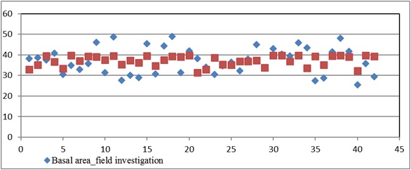
Fig. 4 Comparison of predicted and estimated basal areas
| Index | Equation | Significance | Region applied |
| Basal area (BA) (m)^2 | (DBH)^2/4 pi | To estimate basal area from DBH values | All |
| Biomass (T/Ha) | (2.81+6.78*BA) | Effective for semi evergreen, moist deciduous forest cover types and having moderate rainfall | Coastal |
| Biomass (T/Ha) | (21.297-6.953(DBH))+0.740((DBH)^2 ) | Effective for wet evergreen, semi evergreen forest cover types and having higher rainfall | Sahyadri Interior |
| Biomass (T/Ha) | exp{-1.996+2.32*log((DBH))} | Effective for deciduous forest cover types and having lower rainfall | Plains |
| Carbon stored (T/Ha) | (Estimated biomass)*0.5 | Sequestered carbon content in the region by forests | All |
| Annual Increment in Biomass (T/Ha) | (Forest cover)*6.5 (Forest cover)*13.41 (Forest cover)*7.5 |
Incremental growth in biomass(Ramachandra et al. 2000) | Coastal Sahyadri Plains |
| Annual increment in Carbon (T/Ha) | (Annual Increment in Biomass )*0.5 | Incremental growth in carbon storage | All |
| Net annual Biomass productivity (T/Ha) | (Forest cover)*3.95 (Forest cover)*5.3 (Forest cover)*3.5 |
Used to compute the annual availability of woody biomass in the region. (Ramachandra et al. 2000) | Coastal Sahyadri Plains |
| Carbon sequestration of forest soil (T/Ha) | (Forest cover)*152.9 (Forest cover)*171.75 (Forest cover)*57.99 |
Carbon stored in soil(Ravindranath et al. 1997) | Coastal Sahyadri Plains |
| Annual Increment of soil carbon | (Forest cover)*2.5 | Annual increment of carbon stored in the soil | All |
Table 1 Biomass computation for different agro zones (Ramachandra et al. 2000a, b)
| Slno | Vegetation types | Biomass (t/ha/year) |
| 1 | Dense evergreen and semi evergreen | 13.41 to 27.0 |
| 2 | Low evergreen | 3.60 to 6.50 |
| 3 | Secondary evergreen | 3.60 to 6.50 |
| 4 | Dense deciduous forest | 3.90 to13.50 |
| 5 | Savanna woodland | 0.50 to 3.50 |
| 6 | Coastal (scrub to moist deciduous) | 0.90 to 1.50 |
Table 2 Biomass productivities in various types of vegetation
2.2.4 Forest plantations
Afforestation activities are aimed at removal of emissions through improved carbon sequestrations with a green cover. Mitigating the carbon content from the atmosphere through the establishment of forest plantation on wastelands, community lands and in agricultural land (Gera et al. 2003) would not only help in fulfilling the target of maintaining the green cover but also mitigation of changes in the climate (Buma and Wessman 2013), but unplanned intensified monoculture plantations have impacted the biodiversity (Gibson et al. 2011). Rapid conversion of forests for timber production, agriculture, and other uses has caused serious consequences on the ecology and biodiversity (Laurance et al. 2012). Monoculture plantations are associated with relatively low ecological values and may be vulnerable to disturbances caused by anthropogenic activities induced climate change. The expansion of monoculture plantations with the decline of native forest cover, has accentuated extinction risk for many forest-dependent taxa (Chapin et al. 2007) and also led to an increase in the acidity of soils, with long-term associated consequences for biodiversity and subsequent land cover (Jonsson et al. 2003; Felton et al. 2010). Carbon sequestration by monoculture plantations was estimated based on field measurements as well as published literatures. The comparative analyses of carbon uptake by the native forests with the monoculture plantations highlight the supremacy of natural vegetation in carbon sequestration.
2.2.5 Forest Soils
Forest soils are major sinks of carbon, approximately 3.1 times larger than the atmospheric pool of 800 GT (Oelkers and Cole 2008). The carbon is stored in the soil as soil organic matter (SOM) in both organic and inorganic forms. SOM input is determined by the root biomass and litter (Jandl et al. 2007). SOM is a complex mixture of carbon compounds, consisting of decomposing plant and animal tissue, microbes (protozoa, nematodes, fungi, and bacteria), and associated soil carbon minerals. SOM improves soil structure, enhances permeability while reducing erosion, with bioremediation leads to the improved quality in groundwater and surface waters. Soil disturbance through deforestation also leads to increased erosion and nutrient leaching from soils (Bruun et al. 2015), which have led to eutrophication and resultant algal blooms within inland aquatic and coastal ecosystems, ultimately resulting in dead zones in the ocean (Ontl and Schulte 2012). Soil carbon is calculated based on the field estimations in top 30 cm soil for different forests (Table 3) and mean soil carbon reported in literature (Ravindranath et al. 1997).
| Slno | Forest Types | Mean soil carbon in top 30 cm (Mg/ha) |
| 1 | Tropical Wet Evergreen Forest | 132.8 |
| 2 | Tropical Semi Evergreen Forest | 171.7 |
| 3 | Tropical Moist Deciduous Forest | 57.1 |
| 4 | Littoral and Swamp Forest | 34.9 |
| 5 | Tropical Dry Deciduous Forest | 58 |
| 6 | Tropical Thorn Forest | 44 |
| 7 | Tropical Dry Evergreen Forest | 33 |
Table 3 Soil carbon storage in different forest types
2.2.6 Estimation of sector-wise carbon emissions
Carbon budgeting at the district level has been done considering ecosystem-wise carbon sequestration potential and sector-wise emissions using multiple data sets. Sector wise carbon emissions were compiled from literature (Ravindranath et al. 1997; Ramachandra et al. 2000a; Murali et al. 2005; Ravindranath et al. 2008) and review of the emission experiments (Ontl and Schulte 2012).
2.2.6.1 Livestock
Livestock is an important component of an agroecosystem, provides the critical energy input to the croplands required for ploughing, threshing and other farm operations. Animal dung used in the manufacture of organic manure provides the essential nutrients that enrich soil fertility and crop yields. Livestock produces methane (CH4) emissions from enteric fermentation. CH4 and N2O (nitrous oxide) emissions are from livestock manure management systems and agriculture sector accounts approximately 20 and 35% of the global GHG emissions. The enteric fermentation in livestock alone accounts for nearly 70% of the global CH4 emission (Eggleston et al. 2006; Gas 2006). Methane emission assessment has been done for the district based on the emission factor details available at Indian emission inventories of GHG (Garg et al. 2001a, b; Kumari et al. 2014). CH4 emission factors of Indian livestock is based on dry matter intake (DMI) approach for different animal categories and methane conversion factors were based on the feeding experiments (Singhal et al. 2005; Gupta et al. 2007). Methane emissions varied from 0.8 to 3.3 kg CH4/animal/year and N2O emission factors were varied from 3 to 11.7 mg/animal/year, which are lower than the IPCC default values. GHG emissions from livestock through enteric fermentation methane emission factor (EFT) were calculated following IPCC, 2006 chapter 10-11 (Eggleston et al. 2006). Livestock population (Census 2011) data was obtained from the State Veterinary Department, Government of Karnataka (Annexure-1, Table A). Siddapur, Sirsi, Joida and Yellapura are the potential regions for dairy development. Livestock density (equation 5) is computed village wise as per the equation 5.
D=Pi/A ....5
where, D is Livestock density, Pi is Livestock population and A is Area of the region. Methane emissions due to the enteric fermentation are computed as per equation 6, based on Tier 1 (Eggleston et al. 2006).
CH4 Enteric =ΣT(EFT*NT)/106 ....6
where, CH4 Enteric is CH4 emissions from enteric fermentation, Gg CH4/yr; EFT is emission factor for the defined livestock category, kg CH4/animal/year; NT is the number of animals of livestock for category T; T is a category of livestock. EFT for various livestock categories is listed in Annexure-1, Table B.
Emission factors for manure depend on the manure volatile solids content, temperature and manure management practices. The emission factors EFT (for various average annual temperature) are given by IPCC for the respective livestock categories [46]. Methane emissions due to manure management is estimated as per equation 7,
CH4 Manure =ΣT(EFT*NT)/106 ....7
where, CH4 is methane emissions from manure (Gg CH4/yr) by area; EFT is emission factor for the defined livestock category, kg CH4/animal/year by region; NT is the number of head of livestock for category T in the region; T is category of livestock. Emission factors based on earlier field estimates were used to compute category wise emission. Emission factor 2.83 to 76.65 kg CH4/animal/year (Annexure-1, Table C) for enteric fermentation. Emission factor of 0.8±0.04 to 3.3±0.16 kg CH4/animal/year was considered for manure management of bovines and 0.1 to 6 kg CH4/animal/year for non-bovines.
2.2.6.2 Agriculture (paddy cultivation)
Agricultural sources are the largest global source of non-CO2 emissions. Globally, 70% of methane emission was contributed by six anthropogenic sources and 20% of methane emission was contributed by paddy (Oryza sativa or Oryza glaberrima) cultivation. Methane is emitted from water stagnant paddy fields due to anaerobic fermentation of organic soil and is transported through rice plants, contributes around 20% of the global methane budget (Zhang et al. 2016). CH4 emissions are estimated by multiplying daily emission factors (Eggleston et al. 2006) by cultivation period of rice and annual harvested areas. Rice is a staple food and is grown in almost all villages, which occupies 30% of the total cropped area in the district. Rainfed water logged category of paddy fields constitutes 41% of the total harvested area and methane emission is computed as per equation 8,
CH4 Rice=(EF*t*A) ....8
Where, CH4 Rice is the annual methane emissions from rice cultivation, Gg CH4/yr; EF is a daily emission factor for kg CH4/ha/day; t is cultivation period of rice; A is an annual harvested area of rice ha/yr. The EF was considered as 0.45 Tg/Y [54].
2.2.6.3 Fuelwood consumption
Energy is a fundamental and strategic tool even to attain the minimum quality of life. The procurement of energy is also responsible in varying degrees for the ongoing deforestation, and loss of vegetation and topsoil (Matrinot 2013; Bailis et al. 2015). CO2 released through incineration occurs at a much faster rate than decomposition because burning wood takes a few seconds and decomposition takes years. Inefficient and incomplete combustion of wood can result in elevated levels of greenhouse gases other than CO2. The energy content of wood ranges from 14.89 to 16.2 megajoules per kilogram (4.5 to 5.2 kWh/kg). Per Capita Fuel Consumption (PCFC) values (Table 4, computed as per equation 9) were analyzed to account fuel consumption pattern in various agro-climatic zones of the Uttara Kannada district and determine the carbon emissions due to fuelwood consumption at domestic level.
PCFC=FC/Σ(Ai) ... 9
Where PCFC is per capita fuel consumption; FC is fuel consumed in kgs/day and Ai is number of adult equivalents, depending on the number of individuals and the age group (i = 1 for adult male, 0.8 for adult female, 0.6 for children (age group 6-18), 0.4 for children), for whom food was cooked. The emission is computed based on the field data of fuelwood consumption (Revised, 1996; Ramachandra et al. 2000; Ramachandra et al. 2014) as per equation 10,
Carbon dioxide emission=(No of households *PCFC*emission factor) ....10
| Agro-climatic Region | Cooking fuelwood (kg/person/day) | Cooking fuelwood (tons/person/year) | |||||||
|---|---|---|---|---|---|---|---|---|---|
| Summer | Monsoon | Winter | Average | ||||||
| Avg | SD | Avg | SD | Avg | SD | Avg | SD | ||
| Coastal | 1.98 | 1.40 | 1.95 | 1.34 | 2.11 | 1.73 | 2.01 | 1.49 | 0.734 |
| Plains | 2.02 | 1.34 | 2.22 | 1.38 | 2.32 | 1.59 | 2.19 | 1.44 | 0.8 |
| Sahyadri | 2.22 | 1.56 | 2.23 | 1.94 | 2.51 | 2.77 | 2.32 | 2.09 | 0.85 |
Table 4 Season and region wise cooking
fuelwood requirement(PCFC)(Ramachandra et al. 2000; Cummings et al. 2002)
2.2.6.4 Transportation sector
The basic infrastructures required for the region's economic growth are roads, railways, and water and air connectivity. The demand for infrastructure augmentation increases with the region's pursuit of development goals. The major pollutant emitted from transport are Carbon dioxide (CO2), Methane (CH4), Carbon monoxide (CO), Nitrogen oxides (NOx), Nitrous oxide (N2O), Sulphur dioxide (SO2), Non-methane volatile organic compounds (NMVOC), Particulate matter (PM) and Hydrocarbon (HC). India stands at third biggest in crude oil consumption after China and USA. The transport sector in India consumes about 22% (56.1 mtoe: million tons of oil equivalent) of total energy (255 Mt) (Sakthi and Muthuchelian 2014). Vehicular emissions account for about 60% of the GHG's from various activities in India (Ramachandra et al. 2015b). Taluk wise transport details were collected (Annexure-1, Table E), where Karwar has the highest number of goods vehicles and auto rickshaws. Sirsi has the highest number of vehicles (32184) followed by Karwar with 26820 vehicles. Region specific emission factors based on the type of vehicle are compiled from various literature including regulatory agencies (Reddy and Venkataraman 2002; Garg et al. 2006; Ramachandra and Shwetmala 2009; CPCB 2010; Mittal et al. 2012) (Annexure-1, Table E). Vehicular emissions are calculated as per equation 11,
Ei=Σ(Vehj *Dj)*Eij km ....11
Where, Ei is the emission of the compound; Vehj is Number of vehicles per type (j); Dj is Distance traveled in a year per different vehicle type (j); Eij km is Emission of compound (i) from vehicle type (j) per driven kilometer.
|
3. Results and Discussion
The source wise carbon stock and sector wise emissions have been computed for district level carbon budgeting. Land uses were analyzed using remote sensing data and emission factors from various sources were compiled. Land uses in Uttara Kannada region during 1973 to 2018 are depicted in Fig. 5, which indicates the region now has the evergreen cover of 29.23%, moist deciduous forests account 16.07%. Plantations constitute 18.03% and Horticulture covers 5.17%. The overall accuracy of classification is 82.52, 84.29, 90.0, 90.96 %, with Kappa values of 0.81, 0.83, 0.88, 0.89 respectively for 1973, 1999, 2016 and 2018. Temporal analyses of LU reveal the trend of deforestation, evident from the reduction of evergreen-semi evergreen forest cover from 67.73% (1973) to 29.5% (2018) due to unplanned developmental activities and intensification of plantations. The transition of evergreen-semi evergreen forests to moist deciduous forests is observed with increase in plantations (such as Acacia auriculiformis, Casuarina equisetifolia, Eucalyptus spp., Tectona grandis etc.) constitute 16%. Human habitations have increased during the last four decades, evident from the increase of built-up area from 0.38% (1973) to 5.23% (2018). During 1973 to 2018, the district has witnessed about 398963 ha loss of evergreen forests. Rapid LU changes are observed due to increased agriculture to meet the growing demand of population and large-scale developmental activities in the heart of evergreen forest cover. The deforestation has increased due to various anthropogenic activities, impacting the local ecology and increasing carbon emissions.
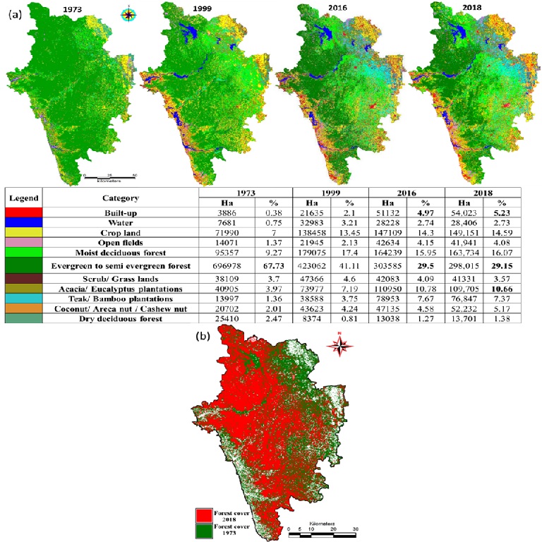
Fig. 5 Land uses and transition of forest cover from 1973 to 2018 in Uttara Kannada
3.1 Carbon Sequestration by forests
Biomass and carbon sequestration were estimated for each grid based in forest category (Fig. 6a, 6b) with the help of biomass data. Sahyadri region shows higher standing biomass (>300 tons/Ha) due to the spatial extent of forests and in particular interior forests. In contrast to this, grids in the coastal and plains taluks have moderate and lower values of biomass per hectare. The total standing biomass of the district is 118627.58 Gg. Grids in the Sahyadri region have higher storage of carbon than the other two regions (Fig. 7a, 7b). Sahyadri region (Supa, Sirsi, Yellapura) have a higher biomass of >1200 Gg. Coastal region (Karwar, Ankola, Kumta, Honnavar) is with moderate biomass. The plains and part of coastal regions are with the lower biomass (< 200 Gg) due to higher forest degradation. The plains taluks mainly consist of agriculture lands, built-up environments and sparse deciduous forest cover. Carbon sequestered by forests accounts to 59313.8 Gg, forests in Supa, Yellapura, Sirsi regions have stored higher carbon (600-800 & >800 Gg) compared to the plains and part of coastal regions. Sahyadri region with protected areas and 'sacred kan' forests have sequestered higher carbon, emphasize the need for protecting sacred forests to mitigate impending changes in the climate due to global warming.
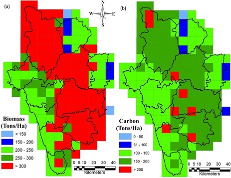
Fig. 6 Biomass estimate and Carbon sequestrated per hectare
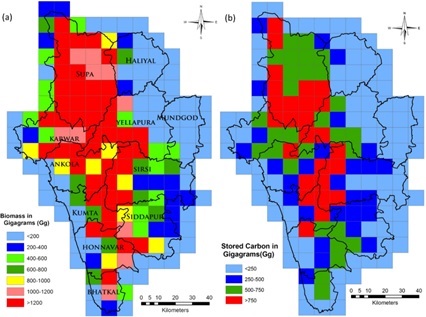
Fig. 7 Biomass estimated and Carbon sequestrated in Gg
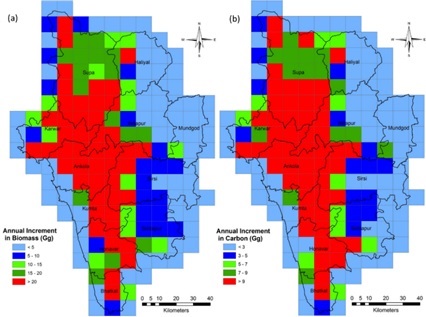
Fig. 8 Annual increment in biomass and carbon (Gg)
Bioenergy availability from forests is assessed as 80-85% population in this region (Ramachandra et al. 2014) depends on fuelwood as a major source for cooking, heating, etc. Fuelwood demand is quantified for each grid considering the population and the annual PCFC (0.77 tons/person/year). The population density for each grid as per 2011 population census (Annexure-1, Fig. i) used for computing supply (availability) to demand ratio is computed to assess the bioenergy status in each grid, considering the annual biomass productivity and fuelwood demand in each grid. The supply (availability) to demand ratio is computed to assess the bioenergy status in each grid, considering the annual biomass productivity (Fig. 9a) and fuelwood demand in each grid. The bioenergy status of the district refers to the ratio of bioenergy availability to the demand. The ratio less than one indicates of fuelwood scarcity situation, while the ratio greater than one indicates of adequate availability of fuelwood. The supply to demand ratio (Fig. 9b) shows Supa taluk is having higher ratio revealing surplus biomass availability due to higher forest cover and lower demand. The central parts of grids (Karwar, Ankola, Sirsi) also show higher availability due to the higher forest in those regions whereas, towards the west in Karwar, Ankola and east part of Sirsi region shows lower ratio due to higher demand (presence of a larger population). Bhatkal, Haliyal, Mundgod and eastern part of Yellapura and Siddapur have the scarcity of resources evident from the supply to demand ratio less than one. Fuelwood scarcity is evident in thickly populated plains and coastal taluks, necessitating the policy interventions to augment bio-resources apart from viable energy alternatives.
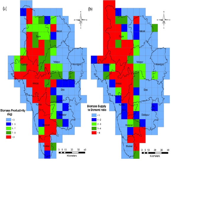
Fig. 9 Annual biomass productivity (deadwood, twigs, fallen branches, etc.) in Uttara Kannada (Gg) and
supply to demand ratio based on population
Soil carbon constitutes the biggest terrestrial carbon pool. The net storage of forest soil carbon in Uttara Kannada district is 59693.44 Gg and Fig. 10a gives grid-wise carbon sequestered in forest soil. The annual increment of 958.81 Gg is depicted grid wise in Fig. 10b. The taluk wise carbon sequestration by forest soils depicts Supa (18585.35 Gg), Ankola (7460.48 Gg), Sirsi (7469 Gg) and Yellapura (6331.05 Gg) have higher soil carbon due to good tree vegetation cover in the region. Bhatkal (1637 Gg) and Mundgod (595.49 Gg) taluks have very low soil carbon due to deforestation.
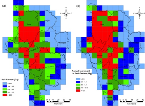
Fig. 10 Annual carbon sequestration and annual increment in soil
3.2 Biomass estimation in forest plantations
Field based estimates were carried out to compare the carbon sequestration potential in native forest and managed plantations in hilly regions of Uttara Kannada district. The spatial extent of forest plantations (land use analysis) is computed for each grid (Fig. 11a). The field based estimates of transect data provided the status of biomass (77.54 t/ha). This is compared with the earlier estimates and used to estimate biomass as well as carbon stored in each grid of the district. The total accumulated biomass of Uttara Kannada district from forest plantation accounts to 14228.08 Gg (Fig. 11b). The spatial extent of forest plantations of Acacia, Eucalyptus, Teak, other hard and softwood plantations ranges from 25957 hectares (Mundgod) to 27426 (Sirsi), 37007 (Haliyal) and 49703 hectares (Yellapura). Haliyal, Yellapura, Mundgod, Sirsi taluks are with higher biomass (>125 Gg) while Siddapur and Kumta have moderate biomass (75-125 Gg). The carbon sequestered in plantations is about 7441 Gg. Higher carbon storage is in plantations of Haliyal, Yellapura, Mundgod, Sirsi (> 60 Gg) while native vegetation has carbon of 100 to 250 Gg. Annual increment in forest plantation biomass in the district is about 1055.55 Gg/yr (Fig. 12a) and carbon is 527.77 Gg/yr (Fig. 12b). Haliyal (Biomass > 12; carbon >9 Gg), Yellapura (> 12; >9 Gg), part of Mundgod (> 12; >9 Gg) have a higher annual increment in biomass as well as carbon. Fig. 13a reflects the carbon stored in soils of plantations. The annual increment in carbon by the soil of forest plantations given in Fig. 13b shows that Haliyal, Yellapura, Mundgod have greater than 6 Gg due to the higher area under plantations. As compared with natural forests plantations did not shown any significant values of CO2 sequestration. In absence of forests, plantations can be considered an alternative solution to fix carbon.
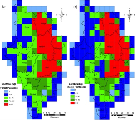
Fig. 11 Biomass and sequestration from forest plantations
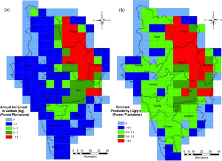
Fig. 12 Annual increment in carbon, biomass productivity from plantations

Fig. 13 Carbon sequestration in soil and annual increment in carbon from plantations
3.3 Carbon emissions
Livestock management in Uttara Kannada offers opportunities for reducing GHG emissions through biogas production form readily available source of manure to replace fossil fuel or forest wood usage. Methane emissions from manure management tend to be smaller than enteric emissions. Two scenarios (Low and High) were considered to analyze potentiality of the region. Tables 5.1 and 5.2 list methane emissions from enteric fermentation and manure (under high as well as lower case scenarios) respectively. Methane from animal wastes is an alternative viable rural energy, provided sufficient feedstock. Energy and biogas potential of livestock residues of all major groups of animals were estimated based on the livestock population (2011). It was seen that Sirsi, Honnavar and Siddapur had the highest biogas potential. Analyses reveal that the domestic energy requirement can be met by biogas option in 428 villages in Uttara Kannada district for more than 60% population. This highlights of optimal use of resources (animal residues) for energy (biogas generation) as well as manure.
| Taluks | Number of animals (B) | Emissions from enteric fermentation(t/yr)(Eef= B*EFT) | Emissions from manure (t/yr)Ema= B* EFT | Total emissions (Eef+Ema) | |
|---|---|---|---|---|---|
| (Tonnes/yr) | Gg/Yr | ||||
| Ankola | 44154 | 724.48 | 173.53 | 898.00 | 0.90 |
| Bhatkal | 3726 | 611.48 | 146.46 | 757.94 | 0.76 |
| Haliyal | 72908 | 1196.27 | 286.53 | 1482.80 | 1.48 |
| Honnavar | 64189 | 1053.21 | 252.26 | 1305.48 | 1.31 |
| Karwar | 25451 | 417.60 | 100.02 | 517.62 | 0.52 |
| Kumta | 53585 | 879.22 | 210.59 | 1089.81 | 1.09 |
| Mundgod | 51829 | 850.41 | 203.69 | 1054.10 | 1.05 |
| Siddapur | 71227 | 1168.69 | 279.92 | 1448.61 | 1.45 |
| Sirsi | 88413 | 1450.68 | 347.46 | 1798.14 | 1.80 |
| Supa | 33778 | 554.13 | 132.72 | 686.85 | 0.69 |
| Yellapura | 52134 | 855.41 | 204.89 | 1060.30 | 1.06 |
| Uttara Kannada | 594929 | 9761.60 | 2338.07 | 12099.67 | 12.10 |
Table 5.1 Emissions from enteric fermentation and manure (High case Scenario)
| Taluks | Number of animals (B) | Emissions from enteric fermentation(t/yr)(Eef= B*EFT) | Emissions from manure (t/yr)Ema= B* EFT | Total emissions (Eef+Ema) | |
|---|---|---|---|---|---|
| (Tonnes/yr) | Gg/Yr | ||||
| Ankola | 44154 | 269.34 | 40.62 | 309.96 | 0.31 |
| Bhatkal | 3726 | 227.33 | 34.29 | 261.61 | 0.26 |
| Haliyal | 72908 | 444.74 | 67.08 | 511.81 | 0.51 |
| Honnavar | 64189 | 391.55 | 59.05 | 450.61 | 0.45 |
| Karwar | 25451 | 155.25 | 23.41 | 178.67 | 0.18 |
| Kumta | 53585 | 326.87 | 49.30 | 376.17 | 0.38 |
| Mundgod | 51829 | 316.16 | 47.68 | 363.84 | 0.36 |
| Siddapur | 71227 | 434.48 | 65.53 | 500.01 | 0.50 |
| Sirsi | 88413 | 539.32 | 81.34 | 620.66 | 0.62 |
| Supa | 33772 | 206.01 | 31.07 | 237.08 | 0.24 |
| Yellapura | 52134 | 318.02 | 47.96 | 365.98 | 0.37 |
| Uttara Kannada | 594929 | 3629.07 | 547.33 | 4176.40 | 4.18 |
Table 5.2 Emissions from enteric fermentation and manure (Low case Scenario)
CO2 emission from fermentation and manure in low case scenario, taluks such as Sirsi, Siddapur Haliyal has the highest CO2 emissions in both processes. The least values are in Karwar, Supa taluks
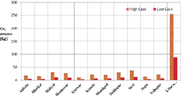
Fig. 14 CO2 emission from livestock in Uttara Kannada
Paddy is grown in two seasons, viz., Kharif (June/July) and rabi or summer (January/February). In all the rice-growing ecosystems, Kharif sowing is common while during the summer season the crop is cultivated mainly in the irrigated areas and the tank-fed areas. In each taluk, nearly 60-80 percent of the total area is covered during Kharif (wet) season while the remaining area is occupied in late Kharif and summer (dry) season. The taluk wise area under paddy cultivation is being shown in Table 6. The total methane emissions from Uttara Kannada paddy cultivation are estimated to be 4.84 Gg/year and its C02 equivalent is 101.57 Gg. Higher paddy cultivation can be seen in Haliyal, Mundgod, Sirsi taluks. The methane emission (Gg) is more in Haliyal (0.90), Mundgod (0.70) Sirsi (0.62) due to the presence of both rainfed and tank based irrigations. The least can be seen in Karwar taluk (0.22) with an area of 3377 Ha under paddy
| Taluks | Area under paddy cultivation (Ha) | Production in tons | Methane emission | Gg CO2 equivalent /Yr. (GWP=21) | |
|---|---|---|---|---|---|
| (T/Yr) | Gg | ||||
| Ankola | 5900 | 17106 | 389.4 | 0.39 | 8.18 |
| Bhatkal | 4270 | 12380 | 281.82 | 0.28 | 5.92 |
| Haliyal | 13705 | 39736 | 904.53 | 0.90 | 19.00 |
| Honnavar | 4559 | 13218 | 300.894 | 0.30 | 6.32 |
| Karwar | 3374 | 9783 | 222.684 | 0.22 | 4.68 |
| Kumta | 5391 | 15706 | 355.806 | 0.36 | 7.47 |
| Mundgod | 10631 | 33117 | 701.646 | 0.70 | 14.73 |
| Siddapur | 6594 | 20029 | 435.204 | 0.44 | 9.14 |
| Sirsi | 9401 | 27898 | 620.466 | 0.62 | 13.03 |
| Supa | 5208 | 15100 | 343.728 | 0.34 | 7.22 |
| Yellapura | 4252 | 15549 | 280.632 | 0.28 | 5.89 |
| Uttara Kannada | 73285 | 219622 | 4836.81 | 4.84 | 101.57 |
Table 6 Taluk wise methane and CO2 emissions from paddy fields
Emission from fuelwood is computed, which shows that the coastal taluks (Karwar, Honnavar, Kumta), Sahyadri taluks (Sirsi and Siddapura), and plains (Haliyal) have higher emissions of carbon. The overall emission from fuelwood consumption of district accounts to be 77.2 Gg. Supa taluk (2.97 Gg) and Yellapura (4.46 Gg) are having least emission values among all taluks (Table 7).
| Coastal region | ||||
|---|---|---|---|---|
| Taluk | No of households(NH) | NH*PCFC(PCFC=2.01 Kg/person/day) | Carbon emission | |
| (T/Yr) | Gg of carbon /year | |||
| Ankola | 21079 | 42368.79 | 5644.58 | 5.64 |
| Bhatkal | 25188 | 50627.88 | 6744.90 | 6.74 |
| Honnavar | 32808 | 65944.08 | 8785.40 | 8.79 |
| Karwar | 35273 | 70898.73 | 9445.48 | 9.45 |
| Kumta | 28251 | 56784.51 | 7565.12 | 7.57 |
| Sahyadri Interior | ||||
| Taluk | No of households(NH) | NH*PCFC(PCFC=2.01 Kg/person/day) | Carbon emission | |
| (T/Yr) | Gg of carbon /year | |||
| Siddapura | 20598 | 45109.62 | 6009.73 | 6.01 |
| Sirsi | 36103 | 79065.57 | 10533.51 | 10.53 |
| Supa | 10186 | 22307.34 | 2971.90 | 2.97 |
| Yellapura | 15292 | 33489.48 | 4461.64 | 4.46 |
| Plains | ||||
| Taluk | No of households(NH) | NH*PCFC(PCFC=2.01 Kg/person/day) | Carbon emission | |
| (T/Yr) | Gg of carbon /year | |||
| Haliyal | 31481 | 73035.92 | 9730.21 | 9.73 |
| Mundgod | 17163 | 39818.16 | 5304.77 | 5.30 |
| Uttara Kannada | 77.2 | |||
Table 7 Agro-climatic region Carbon dioxide emissions from fuelwood consumption
Transportation is another major sector of CO2 emission. The taluk wise vehicle details are analysed and emission from CO2, CO, CH4 is estimated and converted CO2 equivalent. The distance traveled by each vehicle type and emission factors considered are shown in Table 8. The total emission from transportation sector of Uttara Kannada accounts to be 424.9 Gg. The total Carbon dioxide (CO2), Methane (CH4), Carbon monoxide (CO) from Uttara Kannada transport is 396.93 Gg, 1.72 Gg and 3.19 Gg respectively (Table 8). The taluk wise estimate shows Karwar (Gg), Sirsi (Gg) has higher CO2 as well as CO emissions (Fig. 14). The CH4 emissions are more in Yellapura (29.31Gg) Sirsi (24.31Gg), Kumta (23.59 Gg).
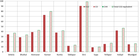
Fig. 15 CO2 emission from transportation in Uttara Kannada
3.4 Carbon budgeting in Uttara Kannada
Carbon budgeting would provide information of Greenhouse Gas (GHG) emissions (especially carbon dioxide (CO2) in the atmosphere, and on the carbon cycle in general), which helps in implementing strategies to mitigate carbon emissions and manage dynamics of the carbon-climate-human system. The ratio of carbon sinks to sources would provide the carbon status in the region. Table 8 and Fig. 15 shows various sources and sinks of carbon in the region at taluk level. The total carbon sequestered from natural vegetation and soil at the district level is 2416.69 Gg. The forest plantation accumulates 963.28 Gg at the district level. The higher accumulation can be seen in Yellapura, Haliyal, Sirsi and Mundgod covering the major part of the region under plantations. Bhatkal, Karwar taluks are showing least values. Carbon status computation (Fig. 16) shows Supa (27.33), Yellapura (14.41), Ankola (6.90) are having higher values revealing the taluks are aiding in higher carbon sequestration as the area under forest cover.
"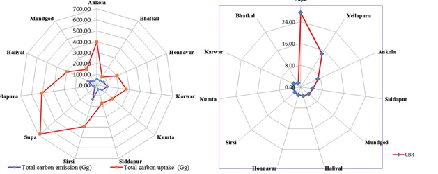
Fig. 16 Taluk wise estimates of carbon sink, sources and carbon status
| Taluk | Emission (CO2equivalent per year) | Carbon uptake (per year) | CBR | ||||||
|---|---|---|---|---|---|---|---|---|---|
| Transport (Gg) | Livestock (Gg) | Agriculture (Gg) | Fuel wood (Gg) | Total (Gg) | Natural forest (Vegetation + Soil) | forest plantation (Vegetation + Soil) (Gg | Fuel wood (Gg Total uptake (Gg)) | ||
| Ankola | 37.22 | 6.51 | 8.18 | 5.64 | 57.55 | 358.03 | 38.91 | 385.94 | 6.90 |
| Bhatkal | 33.76 | 5.49 | 5.92 | 6.74 | 51.92 | 82.65 | 6.08 | 88.72 | 1.71 |
| Honnavar | 42.71 | 9.46 | 6.32 | 8.79 | 67.28 | 174.81 | 31.18 | 31.18 | 3.06 |
| Karwar | 79.70 | 3.75 | 4.68 | 9.45 | 97.57 | 257.51 | 15.92 | 273.42 | 2.80 |
| Kumta | 42.00 | 7.90 | 7.47 | 7.57 | 64.93 | 152.10 | 34.68 | 186.78 | 2.88 |
| Siddapur | 13.39 | 10.50 | 9.14 | 6.01 | 39.04 | 126.15 | 46.46 | 172.61 | 4.42 |
| Sirsi | 99.02 | 13.03 | 10.53 | 135.6 | 255.53 | 139.20 | 394.73 | 2.91 | |
| Supa | 9.80 | 4.98 | 7.22 | 2.97 | 24.96 | 610.67 | 71.58 | 682.25 | 27.3 |
| Yellapura | 17.28 | 7.69 | 5.89 | 4.46 | 35.32 | 238.50 | 270.61 | 509.11 | 14.4 |
| Haliyal | 46.74 | 10.75 | 19.00 | 9.73 | 86.21 | 117.04 | 179.77 | 296.81 | 3.44 |
| Mundgod | 16.27 | 7.64 | 14.73 | 5.30 | 43.95 | 43.71 | 128.91 | 172.62 | 3.93 |
| Uttara Kannada | 437.87 | 87.70 | 101.57 | 77.2 | 704.4 | 2416.69 | 963.28 | 3379.9 | 4.80 |
Table 8 Taluk wise carbon emission and sequestration from various sectors
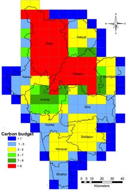
Fig. 17 Carbon status in Uttara Kannada district
4. Acknowledgment
We acknowledge the sustained financial support for ecological research in Western Ghats from (i) NRDMS division, The Ministry of Science and Technology (DST/CES/TVR1045), Government of India, (ii) Indian Institute of Science (IISc/R1011), (iii) The Ministry of Environments, Forests and Climate Change, Government of India (DE/CES/TVR/007), and (iv) Karnataka Biodiversity Board, Western Ghats Task Force, Government of Karnataka We acknowledge the support of Karnataka Forest Department for giving necessary permissions to undertake ecological research in Central Western Ghats. We thank Vishnu Mukri and Srikanth Naik for the assistance during field data collection.
5. Conclusion
Forest ecosystems play a pivotal role in managing carbon in the global carbon cycle, vital habitats of many animal and plant species, retaining water, groundwater recharge, preventing soil erosion and reduction of mud or landslides (as roots help in binding the soil). Based on the detailed investigation and synthesis of biomass resource availability and demand data, the study categorizes the Uttara Kannada district into two zones i.e. biomass surplus zone (consisting of taluks mainly from the Sahyadri Interior) and biomass deficit zone, (consisting of thickly populated plains and coastal taluks such as Bhatkal, Honnavar, Kumta, Mundgod, Haliyal). Total accumulated biomass of natural forest of the district is 118627.54 Gg. The present study reveals the total carbon emitted from major sectors (livestock, paddy cultivation, transportation and fuel consumption) was 704.35 Gg/yr and carbon sequestered is 3379.97 Gg/yr. The taluk wise assessment shows Supa (682.25 Gg/yr), Yellapura (509.11 Gg/yr), Ankola (396.94 Gg/yr) of carbon stored. Least values can be seen in Mundgod, Bhatkal taluks. Supa taluk has a positive carbon status (of 27.33) due to the presence of higher spatial extent of protected forests with moderate disturbances. The least values are in Mundgod, Bhatkal, Haliyal due to higher anthropogenic activities and disturbed forests. Renewable energy technologies are prompted for energy requirement in this ecologically sensitive region as they generate near-zero emissions of GHGs. Generation based incentives would help in the large scale penetration of renewable energy technologies. This would also bring down the local pressure on the forests. Arresting deforestation in ecologically sensitive regions such as the Western Ghats by regulating large scale LU changes and promoting afforestation through the planting of native species are cost effective ways of reducing greenhouse gas emissions and mitigation of impending changes in the climate. Creation of people's nurseries across all regions is encouraged to get ready saplings instead of centralized nurseries of the forest department, which also generate more of rural employment potential. Biomass enrichment is an urgent necessity and poor grade tree plantations of Haliyal, Mundgod, Kirvathi division of Yellapura regions need to be restored with natural forest species through the planting of saplings and seeds to enhance eroded soils. The effective forest management with forest regeneration activities with native species would help in further enhancing carbon status of a region.
|
6. Reference
- Bailis, R., Drigo, R., Ghilardi, A., & Masera, O. (2015). The carbon footprint of traditional woodfuels. Nature Climate Change, 5(3), 266.
- Bharath, S., Rajan, K. S., & Ramachandra, T. V. (2013). Land surface temperature responses to land use land cover dynamics. Geoinformatics Geostatistics: An Overview, 1(4).
- Brown, S. (1997). Estimating biomass and biomass change of tropical forests: a primer (Vol. 134). Food & Agriculture Org.
- Brown, S. L., Schroeder, P., & Kern, J. S. (1999). Spatial distribution of biomass in forests of the eastern USA. Forest Ecology and Management, 123(1), 81-90.
- Bruun, T. B., Elberling, B., Neergaard, A., & Magid, J. (2015). Organic carbon dynamics in different soil types after conversion of forest to agriculture. Land Degradation & Development, 26(3), 272-283.
- Buma, B., & Wessman, C. A. (2013). Forest resilience, climate change, and opportunities for adaptation: a specific case of a general problem. Forest Ecology and Management, 306, 216-225.
- Cairns, M. A., Olmsted, I., Granados, J., & Argaez, J. (2003). Composition and aboveground tree biomass of a dry semi-evergreen forest on Mexico's Yucatan Peninsula. Forest Ecology and Management, 186(1-3), 125-132.
- Chapin III, F. S., Danell, K., Elmqvist, T., Folke, C., & Fresco, N. (2007). Managing climate change impacts to enhance the resilience and sustainability of Fennoscandian forests. AMBIO: A Journal of the Human Environment, 36(7), 528-533.
- Chandran, M. D. S., Rao, G. R., Gururaja, K. V., & Ramachandra, T. V. (2010). Ecology of the swampy relic forests of Kathalekan from Central Western Ghats, India. Bioremediation, Biodiversity and Bioavailability, 4(1), 54-68.
- Ciais, P., Sabine, C., Bala, G., Bopp, L., Brovkin, V., Canadell, J., ... & Jones, C. (2014). Carbon and other biogeochemical cycles. In Climate change 2013: the physical science basis. Contribution of Working Group I to the Fifth Assessment Report of the Intergovernmental Panel on Climate Change (pp. 465-570). Cambridge University Press.
- CPCB. (2010). Status of the vehicular pollution control programme in India. Central Pollution Control Board, Government of India, New Delhi.
- Cummings, D. L., Kauffman, J. B., Perry, D. A., & Hughes, R. F. (2002). Aboveground biomass and structure of rainforests in the southwestern Brazilian Amazon. Forest Ecology and Management, 163(1-3), 293-307.
- Dymond, C. C., Beukema, S., Nitschke, C. R., Coates, K. D., & Scheller, R. M. (2016). Carbon sequestration in managed temperate coniferous forests under climate change. Biogeosciences, 13(6), 1933.
- Edgar. (2011). EDGAR - Emission Database for Global Atmospheric Research. Glob Emiss EDGAR v42, 3720. doi:10.2904/EDGARv4.2.
- Eggleston, S., Buendia, L., & Miwa, K. (2006). 2006 IPCC guidelines for national greenhouse gas inventories [recurso electrónico]: waste. Kanagawa, JP: Institute for Global Environmental Strategies.
- Felton, A., Lindbladh, M., Brunet, J., & Fritz, Ö. (2010). Replacing coniferous monocultures with mixed-species production stands: an assessment of the potential benefits for forest biodiversity in northern Europe. Forest ecology and management, 260(6), 939-947.
- Gallaun, H., Zanchi, G., Nabuurs, G. J., Hengeveld, G., Schardt, M., & Verkerk, P. J. (2010). EU-wide maps of growing stock and above-ground biomass in forests based on remote sensing and field measurements. Forest Ecology and Management, 260(3), 252-261.
- Garg, A., Bhattacharya, S., Shukla, P. R., & Dadhwal, V. K. (2001). Regional and sectoral assessment of greenhouse gas emissions in India. Atmospheric Environment, 35(15), 2679-2695.
- Garg, A., Shukla, P. R., Bhattacharya, S., & Dadhwal, V. K. (2001). Sub-region (district) and sector level SO2 and NOx emissions for India: assessment of inventories and mitigation flexibility. Atmospheric Environment, 35(4), 703-713.
- Garg, A., Shukla, P. A., & Kapshe, M. (2006). The sectoral trends of multigas emissions inventory of India. Atmospheric Environment, 40(24), 4608-4620.
- Gas, G. A. N. C. G. (2006). Emissions: 1990-2020. Office of Atmospheric Programs Climate Change Division US Environmental Protection Agency, Washington, June2006.
- Gera, M., Bisht, N. S., & Gera, N. (2003). Carbon Sequestration Through Community Based Forest Management - a Case Study from Sambalpur Forest Division, Orissa. Indian Forestry, 129, 735-40.
- Gibson, L., Lee, T. M., Koh, L. P., Brook, B. W., Gardner, T. A., Barlow, J., ... & Sodhi, N. S. (2011). Primary forests are irreplaceable for sustaining tropical biodiversity. Nature, 478(7369), 378.
- Gupta, P. K., Jha, A. K., Koul, S., Sharma, P., Pradhan, V., Gupta, V., ... & Singh, N. (2007). Methane and nitrous oxide emission from bovine manure management practices in India. Environmental Pollution, 146(1), 219-224.
- Gupta, P. K., Gupta, V., Sharma, C., Das, S. N., Purkait, N., Adhya, T. K., ... & Singh, G. (2009). Development of methane emission factors for Indian paddy fields and estimation of national methane budget. Chemosphere, 74(4), 590-598.
- Hooijer, A., Page, S., Canadell, J. G., Silvius, M., Kwadijk, J., Wösten, H., & Jauhiainen, J. (2010). Current and future CO2 emissions from drained peatlands in Southeast Asia. Biogeosciences, 7(5), 1505-1514.
- IEA-International Energy Agency. (2010). Energy Technology Perspectives: Scenarios & Strategies To 2050. doi:10.1049/et:20060114.
- Jackson, R. B., & Baker, J. S. (2010). Opportunities and constraints for forest climate mitigation. BioScience, 60(9), 698-707.
- Jandl, R., Lindner, M., Vesterdal, L., Bauwens, B., Baritz, R., Hagedorn, F., ... & Byrne, K. A. (2007). How strongly can forest management influence soil carbon sequestration?. Geoderma, 137(3-4), 253-268.
- Jonsson, U., Rosengren, U., Thelin, G., & Nihlgård, B. (2003). Acidification-induced chemical changes in coniferous forest soils in southern Sweden 1988-1999. Environmental Pollution, 123(1), 75-83.
- Kumari, S., Dahiya, R. P., Kumari, N., & Sharawat, I. (2014). Estimation of methane emission from livestock through enteric fermentation using system dynamic model in India. International Journal of Environmental Research and Development, 4, 347-352.
- Laurance, W. F., Useche, D. C., Rendeiro, J., Kalka, M., Bradshaw, C. J., Sloan, S. P., ... & Arroyo-Rodriguez, V. (2012). Averting biodiversity collapse in tropical forest protected areas. Nature, 489(7415), 290.
- Manua Loa. (2017). n.d. https://www.esrl.noaa.gov/gmd/obop/mlo/, Accessed on May 13, 2017.
- Matrinot, E. (2013). Renewables Global Futures Report (Paris: REN21). Renew Energy Policy Netwrok 21st Century.
- Mittal, M. L., Sharma, C., & Singh, R. (2012). Estimates of emissions from coal fired thermal power plants in India. In 2012 International emission inventory conference (pp. 13-16).
- Mohren, G. M. J., Hasenauer, H., Köhl, M., & Nabuurs, G. J. (2012). Forest inventories for carbon change assessments. Current Opinion in Environmental Sustainability, 4(6), 686-695.
- Murali, K. S., Bhat, D. M., & Ravindranath, N. H. (2005). Biomass estimation equations for tropical deciduous and evergreen forests. International Journal of Agricultural Resources, Governance and Ecology, 4(1), 81-92.
- Oelkers, E. H., & Cole, D. R. (2008). Carbon dioxide sequestration a solution to a global problem. Elements, 4(5), 305-310.
- Ontl, T. A., & Schulte, L. A. (2012). Soil carbon storage. Nature Education Knowledge, 3(10).
- Pachauri, R. K., & Reisinger, A. (2007). Contribution of Working Groups I, II and III to IPCC fourth assessment report. IPCC, Geneva.
- Pan, Y., Birdsey, R. A., Fang, J., Houghton, R., Kauppi, P. E., Kurz, W. A., ... & Ciais, P. (2011). A large and persistent carbon sink in the world's forests. Science, 1201609.
- Pascal, J. P. (1986). Explanatory Booklet on Forest Map of South India. French Institute, Pondicherry, 19-30.
- Pascal, J. P. (1988). Wet evergreen forests of the Western Ghats of India, French Institute, Pondicherry.
- Quere, C. L., Moriarty, R., Andrew, R. M., Peters, G. P., Ciais, P., Friedlingstein, P., ... & Boden, T. A. (2015). Global carbon budget 2014. Earth System Science Data, 7(1), 47-85.Ravindranath, N. H., Somashekhar, B. S., & Gadgil, M. (1997). Carbon flow in Indian forests. Climatic Change, 35(3), 297-320.
- Ravindranath, N. H., & Ostwald, M. (2007). Carbon inventory methods: handbook for greenhouse gas inventory, carbon mitigation and roundwood production projects (Vol. 29). Springer Science & Business Media.
- Ramachandra, T. V., Subramanian, D. K., Joshi, N. V., Gunaga, S. V., & Harikantra, R. B. (2000). Domestic energy consumption patterns in Uttara Kannada district, Karnataka state, India. Energy Conversion and Management, 41(8), 775-831.
- Ramachandra, T. V., Joshi, N. V., & Subramanian, D. K. (2000). Present and prospective role of bioenergy in regional energy system. Renewable and sustainable energy reviews, 4(4), 375-430.
- Ramachandra, T. V., Shwetmala. (2009). Emissions from India's transport sector: Statewise synthesis. Atmospheric Environment, 43(34), 5510-5517.
- Ramachandra, T. V., Hegde, G., Setturu, B., & Krishnadas, G. (2014). Bioenergy: A sustainable energy option for rural india. Advances in Forestry Letters (AFL), 3(1), 1-15.
- Ramachandra, T. V., Chandran, M. D. S., Rao, G. R.,Vishnu, D. M., Joshi, N. V. (2015a). Floristic diversity in Uttara Kannada district, Karnataka, In Biodiversity in India. New Delhi: Regency publications, Delhi.
- Ramachandra, T. V., Aithal, B. H., & Sreejith, K. (2015b). GHG footprint of major cities in India. Renewable and Sustainable Energy Reviews, 44, 473-495.
- Ramachandra, T. V., Setturu, B., Rajan, K. S., & Chandran, M. S. (2016). Stimulus of developmental projects to landscape dynamics in Uttara Kannada, Central Western Ghats. The Egyptian Journal of Remote Sensing and Space Science, 19(2), 175-193.
- Ramachandra, T. V., Bharath, S., & Gupta, N. (2018). Modelling landscape dynamics with LST in protected areas of Western Ghats, Karnataka. Journal of environmental management, 206, 1253-1262.
- Reddy, M. S., & Venkataraman, C. (2002). Inventory of aerosol and sulphur dioxide emissions from India. Part II-biomass combustion. Atmospheric Environment, 36(4), 699-712.
- Regos, A., Ninyerola, M., Moré, G., & Pons, X. (2015). Linking land cover dynamics with driving forces in mountain landscape of the Northwestern Iberian Peninsula. International Journal of Applied Earth Observation and Geoinformation, 38, 1-14.
- Revised, I. P. C. C. (1996). IPCC guidelines for national greenhouse gas inventories. Reference manual, 3.
- Sakthi, K., & Muthuchelian, K. (2014). Energy Sources and their Utilization in Service Sector in Selected Cities of Tamil Nadu, India. International Journal of Innovative Research and Development.
- Sala, O. E., Chapin, F. S., Armesto, J. J., Berlow, E., Bloomfield, J., Dirzo, R., ... & Leemans, R. (2000). Global biodiversity scenarios for the year 2100. science, 287(5459), 1770-1774.
- Sharma, M., Areendran, G., Raj, K., Sharma, A., & Joshi, P. K. (2016). Multitemporal analysis of forest fragmentation in Hindu Kush Himalaya-a case study from Khangchendzonga Biosphere Reserve, Sikkim, India. Environmental monitoring and assessment, 188(10), 596.
- Silva, M. E. S., Pereira, G., & da Rocha, R. P. (2016). Local and remote climatic impacts due to land use degradation in the Amazon "Arc of Deforestation". Theoretical and applied climatology, 125(3-4), 609-623.
- Singhal, K. K., Mohini, M., Jha, A. K., & Gupta, P. K. (2005). Methane emission estimates from enteric fermentation in Indian livestock: Dry matter intake approach. Current Science, 119-127.
- Vinay, S., Vishnu, D. M., Srikanth, N., Chandran, M. D. S., Bharath, S., Shashishankar, A., & Ramachandra, T. V. (2017). Landscapes and hydrological regime linkages: case study of Chandihole, Aghanashini. In proceedings of National Seminare for Research Scholars, Bangalore.
- Wei, T., Dong, W., Yuan, W., Yan, X., & Guo, Y. (2014). Influence of the carbon cycle on the attribution of responsibility for climate change. Chinese science bulletin, 59(19), 2356-2362.
- Zhang, B., Tian, H., Ren, W., Tao, B., Lu, C., Yang, J., ... & Pan, S. (2016). Methane emissions from global rice fields: Magnitude, spatiotemporal patterns, and environmental controls. Global Biogeochemical Cycles, 30(9), 1246-1263.
|
Annexure 1
| Taluk | Livestock Category | ||||||||
|---|---|---|---|---|---|---|---|---|---|
| Cattle | Buffalo | Pig | Sheep | Goat | Rabbits | Dogs | Others | Taluk Total | |
| Ankola | 28570 | 5967 | 0 | 0 | 40 | 2 | 9575 | 0 | 44154 |
| Bhatkal | 24619 | 6094 | 84 | 0 | 110 | 44 | 6316 | 0 | 37267 |
| Haliyal | 41485 | 20820 | 32 | 354 | 3738 | 58 | 6421 | 0 | 72908 |
| Honnavar | 47828 | 8849 | 83 | 18 | 6 | 9 | 7396 | 0 | 64189 |
| Karwar | 11218 | 5460 | 294 55 | 4 | 85 | 257.51 | 8335 | 0 | 25451 |
| Kumta | 35891 | 5820 | 6 | 0 | 18 | 3 | 11847 | 0 | 53585 |
| Mundgod | 32122 | 8686 | 14.73 | 1433 | 3039 | 8 | 6460 | 19 | 51829 |
| Siddapur | 43881 | 18897 | 0 | 128 | 235 | 0 | 8080 | 6 | 71227 |
| Sirsi | 52230 | 18845 | 24 | 673 | 3101 | 44 | 13488 | 8 | 88413 |
| Supa | 19052 | 8224 | 0 | 0 | 843 | 6 | 5647 | 0 | 33772 |
| Yellapura | 30053 | 11007 | 315 | 41 | 860 | 18 | 9838 | 2 | 52134 |
| Uttara Kannada | 366949 | 118669 | 900 | 2702 | 11994 | 277 | 93403 | 35 | 594929 |
Table A The livestock available at category wise of Uttara Kannada region for the year 2011
| Source categories | Details | Emission factors(kg CH4 Animal - 1 yr - 1) |
| Cattle | ||
| Cattle-crossbred (male),4-12 months
Cattle -crossbred (male), 1-3 years Cattle-crossbred (male), 3 years Breeding Cattle-crossbred male, Working Cattle-crossbred (male), Breeding and Working Cattle-crossbred (male), others Cattle-crossbred (female), 4-12 months Cattle-crossbred (female), 1-3 years Cattle-crossbred (female), Milking Cattle-crossbred (female), Dry Cattle-crossbred (female) Heifer Cattle-crossbred (female), others Cattle-indigenous (male), 0-12 months Cattle-indigenous (male), 1-3 years Cattle-indigenous (male,<3 years Breeding Cattle-indigenous (male),Working Cattle-indigenous (male), Breeding and Working Cattle-indigenous (male), others Cattle-indigenous (female),4-12 months Cattle-indigenous female,1-3 years Cattle-indigenous (female), Milking Cattle-indigenous (female), Dry Cattle-indigenous (female), Heifer Cattle-indigenous (female), others |
9.02
19.67 36.14 36.31 34.05 26.07 9.71 21.31 38.83 38.51 21.49 23.6 7.6 16.36 34.86 32.94 29.42 24.37 7.39 15.39 35.97 29.38 22.42 24.1 |
|
| Buffalo | ||
| Buffalo (male),0-12 months
Buffalo (male),1-3 years Buffalo (male),<3 years Breeding Buffalo (male), Working Buffalo (male), Breeding and Working Buffalo (male), others Buffalo (female), (0-1) months Buffalo (female),1-3years Buffalo (female), Milking Buffalo (female),Dry Buffalo (female), Heifer Buffalo (female), others |
5.09
14.78 58.69 66.15 54.28 60.61 6.06 17.35 76.65 56.28 36.81 38.99 |
|
| Goat | ||
|
Goat (male),<1 year
Goat (male), >1 year Goat (female) <1 year Goat (female,<1-year milking) Goat (female),<1 year dry |
2.83 4.23 2.92 4.99 4.93 |
|
| Sheep | ||
| Sheep | 3.67 | |
| Others | ||
| Others | 8.64 | |
| Livestock enteric fermentation (Singhal et al. 2005) | ||
|---|---|---|
Table B Emission factors for enteric fermentation
| Source categories | Details | Emission factors(kg CH4 Animal - 1 yr - 1) |
| Cattle | ||
|
Dairy cattle (crossbred), Adult Dairy cattle (Indigenous), Adult Non-Dairy cattle (Crossbred), 0-1 year Non-Dairy cattle (Crossbred), 1-2.5year Non -Dairy cattle (Crossbred), Adult Non-Dairy cattle (Indigenous), 0-1 year Non Dairy cattle (Indigenous), 1-3year Non Dairy cattle (Crossbred), Adult |
3.3±0.16 2.7±0.13 0.8±0.04 1.7±0.08 2.3±0.11 0.8±0.04 2±0.1 |
|
| Buffalo | ||
|
Dairy buffalo Non-Dairy buffalo, 0-1 year Non- Dairy buffalo, 1-3year Non-Dairy buffalo, Adult |
3.3±0.06 1.2±0.02 2.3±0.04 2.7±0.05 |
|
| Livestock manure management (Gupta et al. 2007) | ||
|---|---|---|
Table C Emission factors for manure.
| Taluks | Motorcycles | Car | Cabs | Auto rickshaws | Omnibuses | Tractors and trailers | Ambulance | Good vehicle | others |
| Ankola | 8141 | 775 | 55 | 341 | 124 | 31 | 10 | 592 | 406 |
| Bhatkal | 16776 | 1056 | 117 | 1078 | 76 | 41 | 6 | 353 | 467 |
| Haliyal | 14705 | 968 | 28 | 289 | 184 | 751 | 11 | 566 | 309 |
| Honnavar | 11479 | 687 | 145 | 449 | 177 | 22 | 8 | 645 | 376 |
| Karwar | 21763 | 1601 | 139 | 1018 | 325 | 85 | 12 | 1129 | 748 |
| Kumta | 12835 | 989 | 159 | 557 | 36 | 22 | 11 | 741 | 534 |
| Mundgod | 4171 | 275 | 11 | 87 | 35 | 574 | 4 | 227 | 105 |
| Siddapur | 4970 | 226 | 12 | 81 | 38 | 90 | 2 | 204 | 94 |
| Sirsi | 26001 | 1792 | 118 | 678 | 316 | 423 | 16 | 1545 | 1295 |
| Supa | 2423 | 400 | 25 | 9 | 39 | 96 | 8 | 89 | 63 |
| Yellapura | 5339 | 304 | 15 | 110 | 35 | 154 | 4 | 293 | 105 |
| Total | 128603 | 9073 | 824 | 4697 | 1385 | 2289 | 92 | 6384 | 4502 |
Table D Taluk wise transport and communication of Uttara Kannada district
| Type of vehicle | Emission factors (g/km) | Reference | ||
|---|---|---|---|---|
| CO2 | CH4 | CO | ||
| Two wheelers for 2001-2005 | 2.2 | CPCB 2010 | ||
| Motorcycles | 26.6 | Mittal and Sharma 2003 | ||
| Motorcycles | 0.18 | EEA 2001 | ||
| Auto rickshaw | 60.3 | Mittal and Sharma, 2003 | ||
| Auto rickshaw | 0.18 | EE, 2001 | ||
| Passenger car gasoline(PCG) | 2 | CPCB 2010 | ||
| Cars | 223.6 | Mittal and Sharma 2003 | ||
| Cars | 0.17 | EEA 2001 | Taxi | 208.3 | Mittal and Sharma, 2003 | Taxi | 0.01 | EEA, 2001 |
| Taxi | 1 | CPCB 2010 | ||
| Buses | 515.2 | Mittal and Sharma 2003 | ||
| Buses | 0.09 | EEA 2001 | ||
| Buses | 3.6 | CPCB 2010 | ||
| Goods vehicles | 515.2 | Mittal and Sharma, 2003 | ||
| Goods vehicles | 0.09 | EEA 2001 | ||
| Trucks | 3.6 | CPCB 2010 | ||
| Light commercial vehicles (LCV) | 5.1 | CPCB 2010 | ||
Table E Emission factors for vehicular emission
.jpg)
Fig. i (a, b) Annual biomass availability in the villages (Gg) and the population density of Uttara Kannada
Citation:
Ramachandra T V, Bharath S, 2019. Global Warming Mitigation through Carbon Sequestrations in the Central Western Ghats. Remote Sensing in Earth Systems Sciences,https://doi.org/10.1007/s41976-019-0010-z
|